
Satyaki Roy, Shimpei Ikeno, and Yuta Suzuki
Global ML-powered methods such as Gradient Boosted Trees for time series
Why do we need global models?
In the last blog post, we saw how to train and forecast individual time series data and aggregate the results. Training forecasting models for each series have many benefits. Lack of contamination from other data sources and better debugging ability/flexibility are advantages of training and forecasting each time series individually. Additionally, some of the traditional statistical methods we saw in the last blog expect individual time series as training data. However, there are advantages of having a global model as well:
- Using cutting-edge machine learning and deep learning algorithms for time series.
- Hierarchical data such as geographies, stores, and SKUs can be represented easily by exploiting a vast sales database of sales histories rather than building a separate model for each product.
- We can use exogenous variables as features and reduce overfitting with regularization techniques. This flexibility increase with Deep Learning models as we can use various data structures as features for our model.
- We need to maintain just one model rather than thousands of models.
We also have seen in terms of forecasting performance that global ML models have started to beat traditional statistical models. For instance, In the latest M-competition(M5) in 2020, the top 5 solutions all used the LightGBM in their winning solution. Our final model also uses LightGBM as a key component of the ensemble model. Although global ML models have some issues as well (we will discuss them in later blogs), we found them to be the most effective forecasting method in terms of performance and time saved.
Our pre-modeling approach
Before modeling, we'll do I. Missing value treatment II. Outlier treatment.
1. Missing value Treatment
Our task is to forecast 39 weeks into the future from 2012-11-02. Although the date of the minimum sale in our training data is 2010-02-05, not all stores or dept have complete sales records during this period. Thus while filling in the dates, we start from the minimum date of the store-dept pair till the maximum date of the training date (which is 1 week before the start of the forecast horizon)

As you can see there are large missing values of some stores-depts, e.g.Store 34 and Dept. 78 has 142 missing values which means only 1 data point for training (we expect 143 weeks for a store-dept pair for complete data). Since we do not know the reason behind the missingness of data, for now, we impute the missing data using two strategies -
- Impute by zeros(assuming the store was shut down or zero demand in the intermittent period).
- Seasonal imputation and carry forwarding
We use both approaches in two models in our ensemble to create more variance in the model forecasts.
2. Outlier Treatment
At first, we found some negative values in the sale data

This may be due to back orders or canceled orders but since we do not know the reason, we simply replace them with zero. Apart from checking data sanity, we must also try to make our dependent variable more normal, and less prone to outliers. Although this is not an assumption for ML models, in our experience this improves performance. Although we did not remove outliers, we tried to reduce the variance of the data and make it more normal. We tried the common data transformations such as square-root, log, and Box-Cox, and we found square-root transformation gave the best results.

As you can see the variance of the data is much lower, and the data looks more normal.
Our modeling solution approach
We created the following process to iterate on improving our solution. This method is useful when creating time series models for thousands of sales histories together.
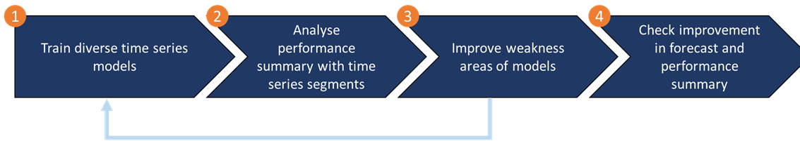
- In step 1, as the fundamental step towards developing a robust ensemble model, we should train strong individual models with different learning capabilities and strengths in terms of bias variance. This will help us reduce the variance in our final ensemble forecast. As you have seen in the previous blog post, we developed multiple statistical models and in this blog post, we will show you how we developed our ML models.
- In step 2, We create a performance summary table per model to check overall performance. At this step, we can remove more models that have poor performance or have taken too much time to train. Then, we create time series characteristics(features) for each individual time series such as entropy, stability, trend, spikes, seasonal strength, etc. Next, create quantiles for each feature and create a performance summary table of each model per quantile of the time series features. Analyzing this table can help us find insights into the relative strength/weaknesses of each time series model.
- In step 3, we will create some new features or new models to improve the weaknesses of our models which we found in step 2.
- Finally, we check our ensemble performance in the validation data.
Post-processing
Finally, we had to make a forecast adjustment that was needed for Christmas.
In our dataset, Christmas Week has 0 pre-holiday days in 2010, 1 in 2011, and 3 in 2012. So, it’s a difference of 3 days from 2012 to 2010 and 2 days from 2012 to 2011. A 2.5-day average, in a week (7 days). So, this is the value that we are going to multiply to Week 51 and add to Week 52 to compensate for what the model didn’t take into account.
Models Considered
- LightGBM, and trend-adjusted LightGBM
- Catboost
- XGBoost
- Random Forest
- Neural Network models(DeepAR, NBEATS, TFT, Vertex AI(AutoML)) [Will bdiscussed in next post]
- Seasonal Auto-ARIMA [Discussed in last blog post]
- Error, Trend, Seasonal (ETS) model [Discussed in last blog post]
- TBATS [Discussed in last blog post]
Comparing the model performance and pros/cons
Table of score and individual rank
| Model | Private Leaderboard Score | Rank | Rank after adjustment |
|---|---|---|---|
| LightGBM | 2585 | 19 | 17 |
| Catboost | 2742 | 37 | 32 |
| XGBoost | 2950 | 112 | 127 |
| Random Forest | 3008 | 135 | 139 |
As you can see, the algorithm selection can make a difference in terms of score. It is not a surprise that LightGBM has emerged as the top choice for most recent time series competitions. XGBoost and Random Forest performs poorly compared to more modern boosting algorithms such as LightGBM and Catboost.
Visual comparison of forecasts
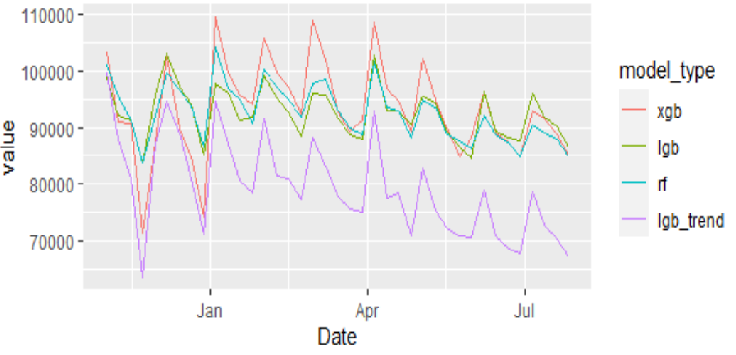
Let us visually inspect some future forecasts for sanity checking.


As you can see, the forecasts for XGBoost are quite noisy, thus we can say that this model is overfitted to the training data. We will thus eliminate this model for the ensemble.
Model weakness - the high trend for tree models
One of the biggest weaknesses of tree-based ML models is the difficulty to capture strong trends. Since tree-based models make predictions based on data splits and the distribution of test data may be significantly different from training data, the forecasts do not capture the strong trend effects. This Store, Dept for e.g. has slowly declining sales.

To capture this trend, we created an additive model called trend-adjusted LightGBM. The design of the model is as follows -
- Train a prophet model on the training data. Use sensible parameters to avoid overfitting trends and change points.
- Extract the trend component and subtract it from the main series. We get the Residuals i.e. trend-adjusted sales, and the predicted trend component.
- We train the LightGBM model on the residuals and predict the residual component of the test period.
- Add the predicted trend component from Prophet and the predicted residuals from LightGBM to get the final forecasts.
Below are the forecasts from the trend-adjusted LightGBM
As we can see, the forecasts are much lower and captured the downward trend of the series. Although these forecasts may be too low or too high and thus should not be used individually, they can be valuable in the ensemble. Another disadvantage of this model is that it is difficult to optimize the hyperparameters of prophet and the ML model together so we had to fix our prophet parameters for each time series.
Although we will have a detailed post on ensembling next time, we can show that just by simply averaging LightGBM and the Trend-adjusted LightGBM, we achieved Rank 3.
| Model | Private Leaderboard Score | Rank | Rank after adjustment |
|---|---|---|---|
| LightGBM | 2585 | 19 | 17 |
| Trend-adjusted LightGBM | 2724 | 36 | 34 |
| Simple Average | 2308 | - | 3 |
Summary
In this blog we discussed our overall modeling process, starting from the data processing to the model building. We shared our process for model improvement and analysis. We saw how just by using the top ML libraries such as LightGBM, we achieved a top 20 rank. Finally, we shared that by combining the strengths and weaknesses of different models we can get effective ensembles - such as the simple average ensemble we showed. This is a preview of more interesting ways of ensembling which we will see in the next post.